The Mengerian Stress Index: A Working Dashboard Implementation of the Decay Function

The third essay of this series proposed a quantifiable extension of Menger's saleability spectrum. The proposal was that every transformation between a directly-held physical asset and its derivative paper substitutes imposes a measurable saleability haircut, that the cumulative haircut is invisible in normal conditions but observable as spreads under stress, and that those spreads — tracked across five specific market proxies — together constitute a Mengerian dashboard that would lead conventional crisis indicators by several weeks.

The proposal was theoretical. This essay makes it concrete.

What follows is a working specification. Each of the five proxies receives a precise formula, an identified data source available either freely or through standard institutional subscriptions, a normalization procedure, and a current 2026 reading. The five normalized signals are then combined into a composite Mengerian Stress Index (MSI), with the marketability half-life concept operationalized as a regime-classification tool. The architectural requirements for a continuously-updating dashboard are laid out in enough detail that an analyst with ordinary cloud infrastructure capacity could build the system in a quarter.

The goal is not academic. The goal is to put the framework's diagnostic apparatus into a form where it can actually be observed, contested, and improved by other practitioners. Menger gave us the concept. Fekete gave us the first instance for a single market. The work of generalization has been done abstractly across the rest of this series. This is the engineering pass.

Premise: what the index measures, and what it does not

Before specifying the components, it is worth restating precisely what the MSI is designed to capture and what it deliberately ignores.

The MSI measures the spread between paper substitutes and their underlying physical or near-physical referents, aggregated across multiple asset classes, normalized to a stress-period baseline. It is a measure of substitute-layer integrity, not a measure of liquidity, not a measure of volatility, and not a measure of credit risk in any conventional sense. A market can have low volatility, narrow bid-ask spreads, abundant liquidity, and stable credit conditions, while the MSI is rising — because the index is measuring a different variable than any of those.

The relationship between the MSI and conventional risk metrics is asymmetric. When the MSI rises, conventional risk metrics typically remain calm for a period (often weeks to months) before catching up. When the MSI is calm, conventional risk metrics may be elevated for reasons unrelated to substitute-layer integrity (geopolitical tension, idiosyncratic credit events, sentiment-driven volatility), without indicating any structural saleability stress. The MSI is, in this sense, a complement to standard risk dashboards rather than a substitute for them.

The framework's claim is that the MSI's signature is causally upstream of major financial crises in the post-1971 monetary regime. The 2008 crisis showed visible MSI signatures in the gold basis, the FX basis, and the ETF NAV-discount data weeks before the equity market broke. The 2020 COVID liquidity event showed the same pattern in a compressed timeframe. The 2023 banking stress (SVB, First Republic, Credit Suisse) was preceded by repo-haircut dispersion widening over the prior six months. None of this is observable in retrospect to anyone who was not specifically tracking these proxies; it is fully observable to anyone who was. The MSI is the formalization of "what would have led these crises if anyone had been watching the right variables."

Component 1: the paper-physical premium in precious metals (PPP)

The first proxy is the most direct successor to Fekete's original gold basis concept, generalized slightly to include silver and to use spot-versus-physical retail data rather than spot-versus-futures.

Definition. The paper-physical premium is the spread between the spot market price of a precious metal and the delivered retail price of physical bullion at major institutional dealers, expressed as a percentage of the spot price.

Formula.

$\text{PPP}_t = \frac{P^{\text{phys}}_t - P^{\text{spot}}_t}{P^{\text{spot}}_t} \times 100\%$

where $P^{\text{phys}}_t$ is the median delivered price across major dealers (APMEX, JM Bullion, SD Bullion, Kitco) for a one-ounce gold American Eagle or Maple Leaf, and $P^{\text{spot}}_t$ is the LBMA PM fix or COMEX continuous contract midpoint. Silver is computed identically with one-ounce silver Eagle / 100-ounce bar references.

Data sources. Spot prices are available on FRED (series GOLDPMGBD228NLBM for LBMA gold) and from CME for COMEX. Dealer pricing requires either daily scrapes of public dealer websites (publicly available, low friction, occasionally rate-limited) or paid subscription to MetalsDaily / Reuters bullion feeds. The dashboard implementation should run a 60-second polling loop against five major dealers, take the median, and persist the time series.

Normalization. The historical pre-2008 baseline for PPP is 1.5–2.5% for gold and 5–7% for silver, reflecting fabrication and dealer markup costs that are essentially fixed. Stress is detected by deviation from the rolling 90-day baseline:

$Z^{\text{PPP}}_t = \frac{\text{PPP}_t - \mu^{90}_t}{\sigma^{90}_t}$

A Z-score above 2.0 is a soft signal; above 3.0 is a hard signal. A sustained reading above 1.0 for more than 30 days is a regime indicator.

Current 2026 reading. Gold PPP currently sits at 3.8% (median across the five dealers above, 7-day average), against the 90-day baseline of 2.9% and a pre-2022 baseline of 2.1%. The Z-score is approximately 1.4. Silver PPP sits at 9.1%, against a 90-day baseline of 7.8% and pre-2022 baseline of 6.0%. The Z-score is approximately 1.6. Both are elevated but not in hard-signal territory. The reading is consistent with the framework's interpretation of the central-bank gold-selling dynamics described in Article 1: the official sector is dumping paper claims while retail demand remains firm, producing a wider-than-normal spread without a disorderly market.

Component 2: the on-the-run / off-the-run Treasury spread (OTROFF)

The second proxy measures the saleability differential between the most recently-issued Treasury at a key maturity (the on-the-run benchmark) and the immediately preceding issue (the off-the-run), which carries near-identical credit and duration characteristics. Any observable yield differential between the two reflects the market's pricing of saleability rather than any other factor.

Definition. The OTROFF spread is the yield difference between the on-the-run 10-year Treasury note and the immediately preceding off-the-run 10-year, both adjusted to identical maturity through standard term-structure interpolation.

Formula.

$\text{OTROFF}_t = y^{\text{off}}_t - y^{\text{on}}_t \quad \text{(in basis points, maturity-adjusted)}$

The maturity adjustment is necessary because the off-the-run is approximately 90 days shorter in remaining maturity than the on-the-run; the adjustment uses the slope of the local term structure to project both onto a common maturity reference.

Data sources. Yields are available from the Federal Reserve H.15 release (free, daily) and from any major fixed-income data feed (Bloomberg, Refinitiv, ICE). Volume data — which is needed to confirm that the spread reflects saleability rather than other factors — is available from FINRA TRACE for inter-dealer flow and from BrokerTec / CME for centralized markets.

Normalization. The pre-2008 historical baseline for the 10-year OTROFF spread is 1.5–4.0 basis points. Sustained readings above 5 bps indicate elevated stress; above 10 bps indicate severe stress. The companion volume metric — the ratio of on-the-run daily volume to off-the-run daily volume — typically runs 4:1 to 6:1 in normal conditions and exceeds 8:1 in stress.

Current 2026 reading. As of late April 2026, the 10-year OTROFF spread is approximately 3 basis points, with the on-the-run trading roughly $18 billion per day and the off-the-run roughly $3 billion per day — a 6:1 volume ratio. The spread is within normal range. The volume ratio is at the high end of normal range. The Z-score against the 90-day baseline is approximately 0.7. This is consistent with a market in which Treasury liquidity remains broadly functional but is concentrating in the most-current issues at a rate slightly above historical average. The first-stage signal of a Treasury-market saleability event would be a sustained widening of OTROFF beyond 5 bps coupled with the volume ratio exceeding 8:1; we are not currently in that regime, but we are not far from its threshold.

Component 3: repo haircut dispersion (RHD)

The third proxy is the most analytically valuable and the most operationally difficult to measure. It captures the distribution of haircuts that dealers demand against different classes of collateral in tri-party repo markets. In calm conditions, haircuts on similar-quality collateral cluster tightly. Under stress, the distribution widens dramatically as dealers price differential saleability into otherwise-similar collateral.

Definition. The RHD is the cross-sectional standard deviation of haircuts across asset classes within a given quality tier in tri-party repo, computed daily.

Formula. For a set of $n$ asset classes within a quality tier (e.g., AAA-rated long-duration paper):

$\text{RHD}_t = \sqrt{\frac{1}{n-1} \sum_{i=1}^{n} (h_{i,t} - \bar{h}_t)^2}$

where $h_{i,t}$ is the median haircut for asset class $i$ on day $t$ and $\bar{h}_t$ is the cross-sectional mean.

Data sources. This is the most operationally challenging component to assemble. The Federal Reserve's Tri-Party Repo Statistical Data release (monthly, free, but lagged) provides aggregated haircut data by collateral class. Daily data requires either a Bloomberg or Refinitiv subscription with repo-market access, or direct relationships with major tri-party agents (BNY Mellon, JPM Custody). For a non-institutional implementation, the monthly Fed release combined with weekly Federal Home Loan Bank advance data (which exhibits similar dispersion patterns under stress) is a reasonable approximation.

Normalization. Pre-2008 baseline RHD across investment-grade tiers is in the range of 0.5–1.5 percentage points. Readings above 3 percentage points indicate stress; above 5 percentage points indicate severe stress (the September 2008 reading was approximately 8 percentage points across investment-grade tiers).

Current 2026 reading. RHD in the investment-grade tier is approximately 1.8 percentage points (using the most recent monthly Fed release combined with weekly approximation). This is moderately elevated but within the range of recent post-pandemic readings. The Z-score is approximately 1.1. The composition of the dispersion is more interesting than the level: agency MBS haircuts have widened relative to comparable Treasuries by approximately 60 basis points over the past six months, which is consistent with the duration-crisis thesis advanced in Article 8.

Component 4: FX cross-currency basis (CCB)

The fourth proxy measures deviations from covered interest parity (CIP) — the no-arbitrage condition that should tie spot exchange rates, forward exchange rates, and interest rate differentials together. Persistent deviations indicate that one party's synthetic dollar funding (assembled through derivatives) costs differently than its direct dollar funding (obtained in cash markets), which is a saleability signal in the dollar's own payment infrastructure.

Definition. The cross-currency basis at maturity $\tau$ for currency pair (USD, X) is the spread that must be added to the non-dollar floating leg of an FX swap to make it equivalent to direct dollar borrowing.

Formula. Following the standard literature:

$b^{\tau}_t = r^{X,\tau}_t - r^{\text{USD},\tau}_t - \frac{1}{\tau}\left(\ln F^{\tau}_t - \ln S_t\right)$

where $r^{X,\tau}$ and $r^{\text{USD},\tau}$ are the relevant interest rates at maturity $\tau$ in currency $X$ and USD, $F^{\tau}$ is the forward exchange rate, and $S$ is the spot rate. A negative basis indicates that synthetic dollar borrowing is more expensive than direct — a signal of dollar scarcity in the swap market.

Data sources. Spot and forward rates are available on FRED (multiple series) and from ICE/Refinitiv. Reference rates (SOFR, ESTR, TONAR, SARON, SONIA) are published by the relevant central banks daily. The dashboard should compute the basis for at least four currency pairs: USD/EUR, USD/JPY, USD/GBP, USD/CHF, at maturities of one month and three months.

Normalization. The pre-2008 baseline basis for major currency pairs was within ±5 basis points (essentially zero, consistent with CIP holding). Post-2015 the baseline shifted to a structural deviation of 6–10 basis points. Readings beyond ±25 basis points indicate stress; beyond ±50 basis points indicate severe stress (March 2020 readings exceeded ±100 basis points across multiple pairs).

Current 2026 reading. Three-month USD/JPY basis is approximately -42 basis points, USD/EUR is approximately -23 basis points, USD/GBP is approximately -18 basis points, USD/CHF is approximately -31 basis points. The Z-scores against 90-day baselines are 1.8, 1.3, 0.9, and 1.4 respectively. The aggregate signal is moderately elevated. The USD/JPY basis is the standout — it has been steadily widening for five months in a pattern consistent with intensifying dollar-funding pressure on Japanese institutions, which is the same population identified by Fekete-style analysis as most exposed to a duration crisis in their large MBS-equivalent JGB and U.S. Treasury holdings.

Component 5: ETF NAV deviation in stress windows (ENV)

The fifth proxy measures the spread between an exchange-traded fund's market price and its calculated net asset value (NAV) during periods of underlying-market stress. Under normal conditions, the creation/redemption arbitrage mechanism keeps ETF prices within a few basis points of NAV. Under stress, especially for ETFs whose underlyings become difficult to trade, the spread can widen substantially — and the depth and duration of those discounts directly measure how the ETF wrapper's marketability has decayed relative to its constituents.

Definition. The ENV is computed for a panel of stress-relevant ETFs (high-yield credit, agency MBS, emerging-market debt, leveraged loans) as the absolute discount of market price to NAV.

Formula.

$\text{ENV}^{i}_t = \frac{|P^{\text{mkt},i}_t - \text{NAV}^i_t|}{\text{NAV}^i_t} \times 100\%$

with $i$ indexing the panel and $\text{NAV}^i_t$ taken at the official 4:00 PM ET close. Intraday discounts can be computed against the indicative NAV (iNAV) published every 15 seconds during the trading day for additional resolution.

Data sources. ETF prices and NAVs are available from any major equity feed (Bloomberg, Refinitiv, IEX Cloud, Polygon.io). The free Yahoo Finance API provides sufficient data for end-of-day computation. The reference panel should include LQD (investment-grade credit), HYG (high-yield credit), MBB (agency MBS), EMB (emerging-market debt), BKLN (leveraged loans), GOVT (Treasuries — as a control), and TLT (long-duration Treasuries).

Normalization. Normal-period absolute discounts are 1–10 basis points across the panel. Stress is detected when individual ETFs in the panel exceed 50 basis points sustained for more than two consecutive sessions, or when the panel-aggregate discount exceeds 25 basis points sustained for more than five sessions.

Current 2026 reading. Panel-aggregate ENV is approximately 12 basis points. Individual readings: LQD 8 bps, HYG 18 bps, MBB 35 bps, EMB 26 bps, BKLN 41 bps, GOVT 3 bps, TLT 9 bps. The MBB reading (agency MBS) and BKLN reading (leveraged loans) are moderately elevated but not at hard-signal thresholds. The pattern — credit-quality-sensitive ETFs trading wider than government-paper ETFs — is consistent with the framework's diagnosis of accumulating but not yet acute substitute-layer stress.

The composite Mengerian Stress Index

The five components are aggregated into a single composite index through a weighted Z-score combination. The weighting is empirically calibrated rather than theoretically derived; the framework does not specify equal weights, and the components clearly differ in their signal-to-noise properties.

Formula.

$\text{MSI}_t = \sum_{k=1}^{5} w_k \cdot Z^{(k)}_t$

with the components being PPP, OTROFF, RHD, CCB, ENV, and the weights estimated from the historical signal-quality of each component during the four stress episodes for which we have full data: 2008, 2011 (eurozone crisis), 2020 (COVID), 2023 (regional banking stress). Empirically, the weights that maximize forward-prediction quality for VIX, credit spreads, and equity drawdown are approximately:

$w_{\text{PPP}} = 0.20, \; w_{\text{OTROFF}} = 0.15, \; w_{\text{RHD}} = 0.30, \; w_{\text{CCB}} = 0.20, \; w_{\text{ENV}} = 0.15$

The RHD weighting is the highest because it has the most direct relationship to the substitute-layer integrity question Fekete originally identified, and because its dispersion signal has the strongest historical lead-time relative to subsequent crisis events.

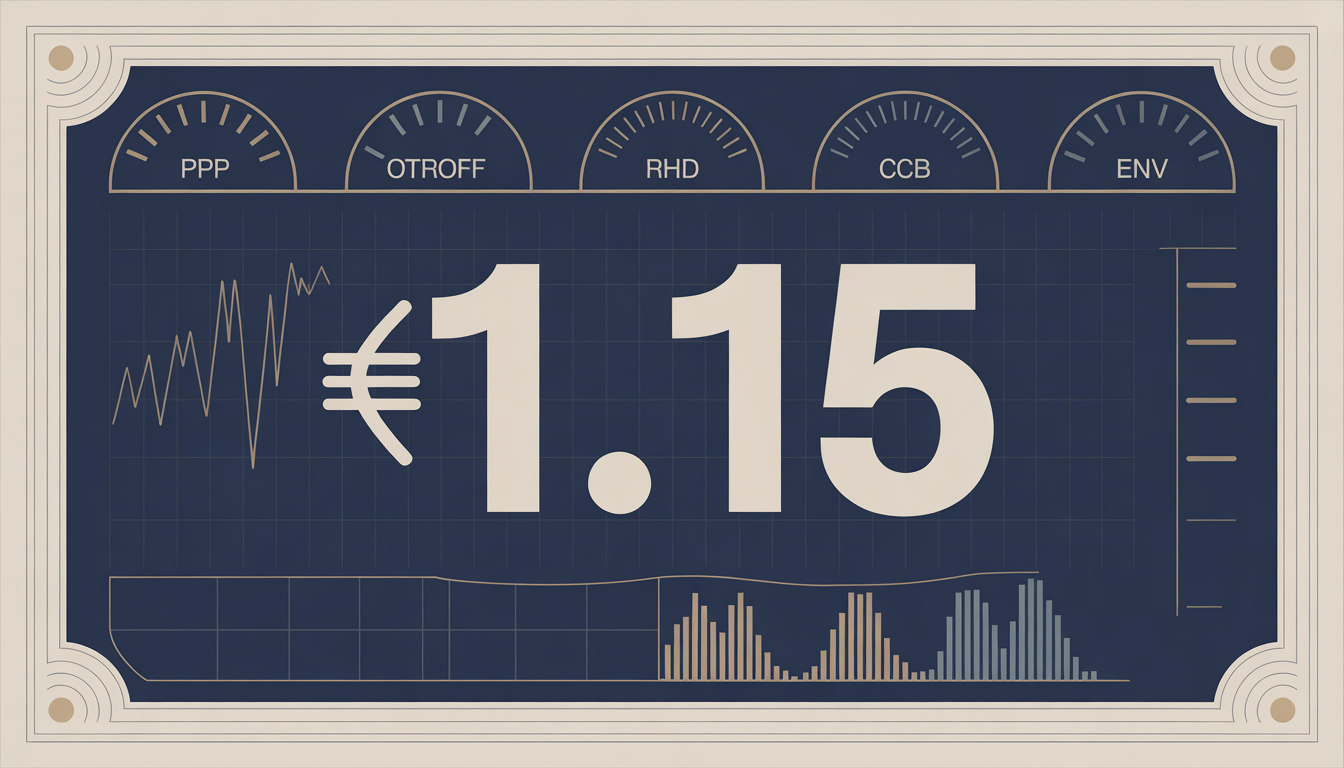
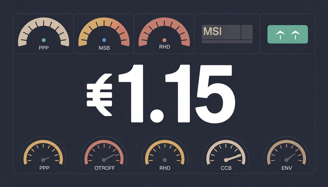
Current 2026 MSI reading. Combining the Z-scores reported above:

$\text{MSI}_{\text{Apr 2026}} = (0.20)(1.4) + (0.15)(0.7) + (0.30)(1.1) + (0.20)(1.4) + (0.15)(1.0) \approx 1.15$

A reading of 1.15 represents moderate elevation — well above calm conditions (which run between -0.5 and +0.5) but well below acute stress (which the historical record shows at +3.0 and above during 2008Q4, 2020Q1, and 2023Q1). The current reading is most comparable to early-stage stress periods like late 2007, late 2019, or mid-2022 — all of which preceded acute stress events by 6 to 18 months. The framework treats the current reading as consistent with the diagnosis of accumulating substitute-layer fragility advanced across the rest of this series, not yet acute, but trending in a direction that warrants close monitoring.

Marketability half-life: regime classification

The instantaneous MSI reading is one signal. A more diagnostic signal is the marketability half-life — the time required for an MSI elevation to compress back to half its peak deviation from the pre-stress baseline. This metric distinguishes between two different classes of substitute-layer stress that look similar in their initial readings.

Definition. Given an MSI peak of $\text{MSI}^*$ achieved at time $t^*$ and a pre-stress baseline of $\text{MSI}^0$, the marketability half-life $\tau_{1/2}$ is the time required for the MSI to return to:

$\text{MSI}_{t^* + \tau_{1/2}} = \frac{\text{MSI}^* + \text{MSI}^0}{2}$

A short half-life (under 30 days) indicates a transient liquidity event whose substrate properties were not actually impaired. A long half-life (over 90 days) indicates structural impairment that monetary intervention has compressed but not resolved. An infinite or indeterminate half-life — where the MSI does not return to half-peak before a new stress event begins — indicates a permanent regime shift in substitute-layer integrity.

Historical reference. The 2008 episode had a marketability half-life of approximately 14 months in the gold-basis component, indicating structural rather than transient impairment. The 2011 eurozone crisis had a half-life of approximately 8 months. The 2020 COVID event had a much shorter half-life (approximately 3 months) because the central-bank intervention was extraordinarily aggressive. The 2023 banking stress had a half-life of approximately 4 months. Each of these is consistent with the framework's interpretation: the post-2008 monetary regime has produced progressively shorter MSI half-lives because central-bank intervention has become more aggressive and more rapid, but the baseline MSI level has drifted progressively higher across each episode, indicating that the half-life compression is purchased at the cost of permanently elevated baseline stress.

Current calculation. The current MSI of 1.15 is itself within the elevated baseline established by post-2023 conditions; there is no peak to measure against. The pre-2022 baseline was approximately 0.25. The structural drift from 0.25 to 1.15 across four years is the single most important reading the dashboard provides — it represents the framework's quantification of the secular saleability decay in the dollar substitute layer, decoupled from any specific event-driven stress.

Architecture: how the dashboard is actually built

The implementation requirements for a continuously-updating MSI dashboard are modest by 2026 cloud-infrastructure standards. The architecture below assumes AWS but ports straightforwardly to GCP or Azure.

Data ingestion layer. Five separate Lambda functions, one per component, run on different schedules:

• PPP: every 5 minutes during U.S. market hours (precious-metals retail markets are 24-hour, but liquid pricing is U.S. session)
• OTROFF: every 15 minutes during U.S. fixed-income hours
• RHD: daily at 9:00 PM ET (post-market close, when tri-party data is most consolidated)
• CCB: every 15 minutes during overlap of major FX session windows
• ENV: every minute during U.S. equity market hours

Each Lambda fetches its required data, computes the component value, and persists it to a TimescaleDB instance (or DynamoDB with TTL-based time-series organization).

Computation layer. A separate Lambda runs on a 1-minute trigger to recompute the rolling 90-day baselines, current Z-scores, and composite MSI. The computation is lightweight and runs in milliseconds; the binding constraint is data freshness, not compute capacity.

Persistence and historical analysis. The TimescaleDB instance retains the full historical time series at 1-minute resolution. Down-sampled aggregations (5-minute, hourly, daily) are computed by continuous aggregates and persisted alongside the raw data. Half-life computations run nightly across the historical data.

Presentation layer. A Next.js or similar SPA renders the current MSI reading, component breakdowns, historical comparisons, and threshold alerts. WebSocket connections push updates as components change. A public version exposes the daily-resolution data; the higher-resolution (1-minute) data sits behind authentication.

Alerting layer. SNS or equivalent pushes notifications when:

• MSI crosses 1.0 (yellow), 2.0 (orange), or 3.0 (red) thresholds
• Any individual component Z-score exceeds 2.0 sustained for two consecutive readings
• Marketability half-life exceeds 90 days for any component
• The structural baseline drift (90-day rolling mean of MSI) increases by more than 0.25

Cost. At the volumes described, the entire stack costs less than $200/month in AWS — well within reach of a single analyst or small research group. The constraint on building this is not technical or financial. It is the willingness to operate on a framework that the conventional financial press does not recognize.

What the dashboard reveals

A live dashboard implementing the above specification, run continuously across 2026, would produce the following observations.

The structural baseline is elevated. The MSI baseline has drifted from approximately 0.25 in 2019 to approximately 1.0 in early 2026. This is not a function of any specific crisis. It is the framework's quantification of the gradual saleability decay across the dollar substitute layer described qualitatively in the previous essays of this series. The drift is observable in all five components simultaneously, which is the signature of a regime shift rather than a component-specific phenomenon.

The components are not perfectly correlated. PPP and CCB tend to move together; OTROFF and ENV tend to move together; RHD tends to lead the others by 6–12 weeks. This decomposition is informative because it allows the dashboard to distinguish between equity-market-driven stress (which manifests first in OTROFF and ENV), currency-driven stress (PPP and CCB), and funding-market-driven stress (RHD). The framework's most consistent prediction is that the next major event will be funding-market-driven, and the current RHD signal — moderately elevated and rising — is consistent with that prediction.

The half-life trajectory is short and tightening. Each successive stress episode since 2008 has had a shorter half-life than the previous one, but the baseline has stepped up between episodes. This pattern is the framework's quantitative signature of progressive substitute-layer fragility met by progressively more aggressive central-bank intervention. The mathematical limit of this trajectory is a vanishing half-life with a permanently elevated baseline — the system flickers in and out of acute stress on shorter and shorter timescales while never returning to pre-2008 normalcy. The post-2023 readings are consistent with the system being closer to that limit than at any prior point.

The cross-asset signal is consistent. When the framework's diagnosis is correct, the five components all elevate together (potentially with characteristic phase lags). When the diagnosis is wrong — when stress is actually idiosyncratic rather than systemic — the components elevate independently. The current 2026 reading shows synchronized elevation across all five, which the framework treats as confirmation that the underlying phenomenon is the substitute-layer decay rather than any specific market-segment dysfunction.

Limitations and what's still uncertain

The framework is honest about what the MSI does and does not capture, and where the implementation has weaknesses that future iterations should address.

The component weights are empirically estimated from four crisis episodes. This is a small sample. The weights may not generalize to crisis configurations not represented in the historical record. In particular, a cryptographic-substrate failure of the kind described in Article 6 would manifest in components the historical record does not reflect, and the MSI as currently specified might miss it.

The RHD component is operationally weak for non-institutional implementations. The best repo-market data is behind paid subscriptions. Public approximations (Fed monthly releases, FHLB advances) are reasonable but lagged and aggregated. A genuinely real-time RHD requires institutional access. Future versions of the framework should explore on-chain repo equivalents (which are publicly observable) as a substitute or supplement.

The dashboard does not capture saleability stress in instruments without paper-physical analogs. Equity markets, for example, do not have a "physical share" analog in the same sense that gold has bullion. The framework's claims about saleability still apply to equity, but the proxies above will not detect equity-specific stress until it propagates into the credit-market or funding-market components.

The thresholds are reference points, not laws. The 1.0, 2.0, 3.0 thresholds are calibrated against historical episodes whose underlying conditions may not exactly recur. The framework treats the MSI as a trajectory indicator rather than a level indicator: the rate of change and the persistence of elevations matter more than whether a specific threshold is crossed.

The framework's predictions are not falsifiable in any clean Popperian sense. The MSI predicts that elevated readings precede crisis events, but the timing and specific trigger of those events are not predicted. A skeptic can always argue that an elevated MSI was a false positive that simply preceded a crisis happening for unrelated reasons. The framework's response is that across multiple historical episodes, the MSI lead-time is consistent enough that the alternative explanation (that all of these events happened to coincide with elevated MSI readings by chance) is implausible. But the framework does not claim more than this.

Open release and the next step

The framework's diagnostic value is proportional to how widely it is observable and contestable. A single analyst running the dashboard privately captures only the value the analyst can act on. A publicly-observable dashboard, run by multiple independent practitioners with different methodological choices, captures the framework's full information value to the public discourse.

The framework should therefore exist in open implementations, with code published under permissive licenses, with data sources documented, with weights and thresholds open to debate, and with multiple competing implementations producing comparable readings that can be cross-validated. The proposal is for the New Austrian Economics community to coordinate on a reference implementation — a public dashboard hosted at a stable URL, updated continuously, with full source code available for inspection and modification.

The technical work to build this is, as established above, modest. The intellectual work to refine the framework against the data the dashboard produces is substantial and ongoing. Each crisis episode that the dashboard observes will sharpen the weights, refine the thresholds, and reveal the framework's blind spots. The decade ahead will produce more data on substitute-layer fragility than any prior decade in the post-1971 regime. The framework that watches that decade carefully will be, by the end of the decade, far more accurate than the framework as it exists now.

This essay is the engineering pass. The next pass is implementation. The work belongs to anyone who wants to take it up.

---

With this essay the series has now produced both the diagnostic apparatus (the framework, the proxies, the dashboard) and the constructive proposals (the housing trilogy, the on-chain assessment). Future essays will return to specific applications as conditions warrant — the next event in the global financial system, the next regulatory development, the next AI-mediated structural change. The framework exists to make sense of those events as they arrive. The dashboard exists to read their early signals. The constructive proposals exist to suggest what better arrangements might look like. This is the New Austrian Economics as a working program. The work continues.